Mitochandrea

Why is it important to know reagent shelf life?

Reagent shelf life is more broadly useful than telling consumers when to expect their milk to sour.

In the biochemical manufacturing and research space, shelf life defines the period over which materials are performing at their prime and what storage temperature maximizes this time. Additionally, shelf life informs when to discard materials and ultimately feeds into upstream processes to optimize batch sizes (no use making more than you can use before expiry, no use making materials more frequently than needed).

Conceptual Overview

Step-by-Step

This page provides the step-by-step experiment and data analysis necessary for calculating your reagent’s shelf life.

Step 1 Determine Method of Testing

Identify the test you will use to determine the performance of your reagent. Typically, this will be some sort of experimental readout, for example, **.

You will need to perform this test over many samples and timepoints, so make sure it is robust – provides sufficient and stable signals. If the variability in your test is high for replicates, it will be difficult to separate signal changes from the noise of your data.

Step 2 Plan:

For any stability study not carried out in real-time, you will need to design your experiment with at least two different storage conditions. The most basic accelerated stability study will include tests carried out at the assigned long-term storage temperature AND at least one higher temperature. For example, if your reagent is typically stored in the fridge (+4C), then your experiment could include samples stored at +4C and room temperature (+21C).

Select your temperatures:

If you are unsure of the optimal storage temperature for your reagent, then include the lowest temperature at which your product can be safely stored. This will ensure that your data tells you the longest possible shelf life that can assigned.

The more temperatures you include, the more confident you can be in your result, but be smart about selecting temperatures that are relevant to your reagent. Do not stray too far from your long-term storage temperature otherwise phenomena that are irrelevant at the storage temperature start to come into play. For example, ice crystal formation at freezing temperatures or protein denaturation at high temperatures.

Typical temperatures include -80C, -20C, 4C, 21C, 37C simply because these are what is readily available with standard laboratory equipment.

Determine the frequency of testing:

The most basic study will include a test on Day 0 to measure 100% performance, then a test on the date of expiry to measure exactly when the product no longer performs to minimum specification. Since it is difficult to know the expiry date ahead of experimentation, especially at accelerated temperatures, you may need to make schedule adjustments while running the study.

Choose timepoints reasonably concentrated around the expected expiry date at the experimental temperature and then one or two timepoints well past the expiry date. These later timepoints will be

For example, if your product is expected to expire in 3 weeks at the experimental (accelerated) storage temperature, then your timepoints could be:

Day 1, 14, 21, 28, and 42.

Your experimental plan will grow more complex as you include additional temperatures with other expected expiry dates and include real-time stability testing.

The estimated shelf life at the long-term storage temperature is:
The estimated shelf life at each of my experimental storage temperatures are:
The timepoints for my study are:

Step 3 Gather your resources:

A good friend of mine once shared some important advice: The best experiment to do is the one you can do.

Don’t fall into the trap of designing your experiment to be so “complete,” that the level of complexity and cost of resources is beyond what is reasonable for the application. At the end of a well-run study, you will know more than you did starting out, which is significantly better than having nothing at all.

Resource	Consideration
Equipment	Check that the equipment used to maintain your samples at the long-term storage and experimental temperatures are within their calibration dates and that you have some redundancy consideration if there is any equipment failure during your study. Ensure that the equipment can be left reasonably undisturbed for the duration of your study. Frequent temperature fluctuations caused by equipment doors opening/closing on shared equipment could harm the quality of your data. If you want to be particularly thorough, use an automated temperature logger to ensure the storage temperatures remain within specification. Although humidity control is preferred, if your equipment cannot control humidity, do not disregard the value of the study. There will be less confidence in your result, but it will still be a meaningful result.
Reagents	Gather sufficient samples for all timepoints to be completed at each timepoint. Don’t forget reagents for the performance tests! Remember to include Day 1, replicates, sufficient samples at your long-term storage temperature to run a real-time study, and overage for any schedule changes or deviated test results that need repeating. I recommend at least 25% overage.
Time	Estimate the time required to complete each performance test for all replicates at each of the required temperatures. Ensure you or someone on your team has sufficient time to complete these studies and puts a reminder in their calendar for each timepoint. Stability studies, especially those that include real-time data, can extend beyond someone’s time of employment, so it is important to document and communicate the planned schedule.

Step 4: Set up Your Data Analysis Template

Learning the theory behind a stability study not only means you understand, but you will make better decisions when things don’t go according to plan.

Step 1 Determine Method of Testing

In this experiment, the reaction of interest is the collision and subsequent degradation of your active reagents, as measured by your performance test. The rate constant for this reaction is referred to as k. You will use the Arrhenius Equation to relate the rate constant at an experimental (typically elevated) temperature (k_exp) to the rate constant at a long-term storage temperature (k_storage) and, ultimately, calculate the expected shelf life at that long-term storage temperature.

For some, now would be a good time to review the associated Excel template.

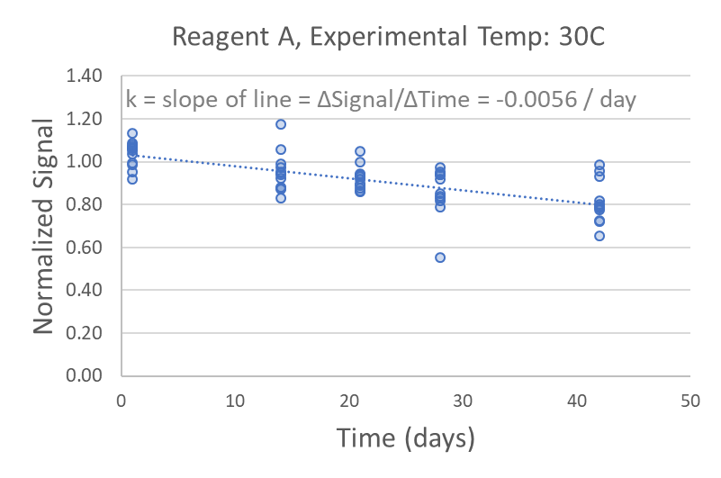
To control for day-to-day experimental variations external to the study, data from each experimental condition is normalized against the long-term storage condition measurements on that day. This should not impact the value of the rate constant, which is calculated as the slope of a linear regression on a Normalized Signal vs. Time plot. If your data is nonlinear, then you have run out your experiment too long and you should truncate your timepoints to stay within the linear range.

Now that you have experimentally determined the rate constant for your experimental temperature (k_exp), you will apply the Arrhenius equation to determine the rate constant for your long-term storage temperature (k_storage)

The Arrhenius equation relates the rate constant (k) to the temperature of the reaction:

k = Aexp(-E_a/RT)

Where A= pre-exponential factor, E_a = activation energy, R = gas constant = 1.987 cal/deg*mole, and T = Kelvin temperature

By setting up the ratio of two Arrhenius equations, we can ultimately solve for k_storage.

k_exp / k_storage = exp(-Ea/R*[1/T_exp – 1/T_storage])

🡪 k_storage =

But wait! We’re still missing the activation energy (Ea), which you can either assume to be an average value or use additional experimental data to calculate. A typical activation energy value in biology is 15000 cal/mol/K. If you have more than two experimental temperatures, then you can use a non-exponential form of the Arrhenius equation and the calculated rate constants to determine your activation energy. The activation energy is solved from a ln(k) vs 1/T plot because the slope is -E_a/R.

ln(k) = ln(A) – Ea/(RT)

With an activation energy value, you can now use the k_storage to determine how long you have before your performance tests signal degrades by X%:

k_storage= Δsignal/Δtime 🡪 shelf-life = Δtime = X/k

Step 5: Go!

Run your first performance test on Day 1 of your experiment. Input your data into the Excel template. Continue running performance tests on the scheduled days and meticulously recording the data.

If you observe any nonlinearity in your data or it seems that you have misjudged your expiry date, take the time to adjust your schedule.

Step 6: Analysis and Conclusion

Example analysis: [link Excel]

Consider the places your shelf life knowledge can be used to inform decisions. Can larger batch sizes be manufactured to reduce repeat manufacturing efforts? Can your reagent be safely stored at an even colder temperature

Step 1 Determine Method of Testing

Select your temperatures:

Determine the frequency of testing:

Resource

Consideration

Equipment

Reagents

Time

Step 1 Determine Method of Testing